Jupyter notebook mode

import numpy as np
import random
import matplotlib.pyplot as plt
from scipy import signal
import scipy
import math

Lecture 2: Noise processes and measurement sensitivity

Expected prior knowledge

Before the start of this lecture, you should be able to:

1. Write down the relation between the autocorrelation function and the power spectral density
2. Describe the power spectral density of white and 1/f noise processes

Learning goals

After this lecture you will be able to:

1. Describe the Poissonian and Gaussian probability distributions and argue when they arise
2. Relate the noise power spectral density of a sensor to its ability to detect a small signal

---

2.1.Where does noise come from?

In general, noise is caused by processes we don't know about, or at least don't know enough about to predict. A good example of this is the Brownian motion of a particle in a liquid, which for the right type of particle, one can even see in a microscope.

Due to random collisions with molecules in the liquid, the particle experiences a randomly fluctuating force: it experiences "force noise", and undergoes random motion in time.

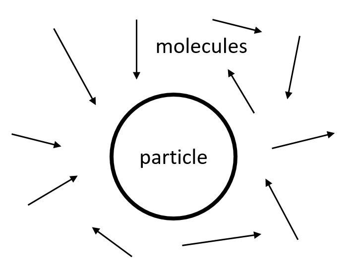
What makes these collision events "random"? Newton's laws certainly are not random. The events are random because we do not have the information needed to predict them: we would need to know the positions and velocities of all the molecules in the liquid. If there are many molecules (large N) and we cannot measure fast enough to observe the motion of the particle in-between collisions then the particle's motion will look random. If we furthermore neglect the time correlations of the motion of the molecules in the liquid, we can describe the random force acting on our particle by the autocorrelation function

$$R_{FF}(\tau) \propto \delta(\tau) \rightarrow S_{FF}(\omega) = \, \text{Constant (white noise)}$$

For such random behavior, what is the probability that if we look at a certain time, we will find the particle at a given position? In other words, what is the probability density function $p(x)$?

In the previous lecture, we drew some cartoons of such distributions with a shape that looked like a Bell curve, corresponding to a Gaussian probability distribution (also called a "normal" distribution): $$p(x) = \frac{1}{\sqrt{2\pi \sigma^2}} e^{-\frac{(x-\mu)^2}{2\sigma^2}}$$

This is a very commonly observed distribution function (hence the name "normal"). The reason it is so common is due to the Central Limit Theorem.

Central Limit Theorem

This theorem tell us that if we

1. collect a large number of independent (uncorrelated) observations/measurements of a statistical quantity
2. calculate the average of these observations
3. repeat steps 1-2 many times to create a collection of averages

then the distribution of the averages will always converge to a Gaussian (normal) distribution in the large $N$ limit. More generally, the central limit theorem tells us that the probability distribution of the sum of many stochastic variables will converge to a Gaussian.

Example: 1D random walk

We consider a particle on a discrete 1D grid. We repeatedly flip a coin and move the particle left or right by one step depending on the outcome of the coin flip. This generates a simplified version of the Brownian motion of a particle. The final position of the particle will be given by the net number of steps in a particular direction.

The probability of finding the particle at a certain final position after $N$ coin flips is described by a Binomial distribution. When $N$ is large, this distribution converges to a Gaussian as described by the central limit theorem.

Note that this is an "unconfined" random walk: the longer we wait (i.e., the larger the number of coin flips $N$), the larger the standard deviation of the distribution will become. We will later also look at the case of a harmonic oscillator. Here the "walk" of the particle is confined by the walls of the potential: the distribution is still Gaussian but now static in time with a width that depends on the average (thermal) energy.

ts = np.linspace(-3,3,100)
def gaussian(ts, mu, sigma):
    return 1/(sigma * np.sqrt(2 * np.pi)) * np.exp( - (ts - mu)**2 / (2 * sigma**2))
plt.plot(ts, 15*gaussian(ts, 0, 1), label="Walker position probability distribution")
plt.plot(ts, [t**2 for t in ts], label="Harmonic confining potential")
plt.legend()
plt.xlabel("Position")
plt.show()

Example: Poisson disribution

If events occur randomly in time at a constant average rate $\lambda$, then the Poisson distribution describes the probability of observing a particular number of events within a time interval $T$. On average, we expect to observe $\mu = \lambda T$ events within this time interval. The probability for observing $n$ events within $T$ is given by $$P(n) = \frac{\mu^n}{n!} e^{-\mu}$$

ns = np.linspace(0,40,41)
def poisson(ns, mu):
    return (np.power(mu, ns) / scipy.special.factorial(ns))*np.exp(-mu)
plt.bar(ns, poisson(ns, 5), label="mu: " + str(5))
plt.bar(ns, poisson(ns, 10), label="mu: " + str(10))
plt.bar(ns, poisson(ns, 20), label="mu: " + str(20))
#plt.plot(ns, poisson(ns, 5), label="mu: " + str(5))
#plt.plot(ns, poisson(ns, 10), label="mu: " + str(10))
#plt.plot(ns, poisson(ns, 20), label="mu: " + str(20))
plt.title("Poisson Distribution")
plt.ylabel("Probability")
plt.xlabel("Number of events")
plt.legend()
plt.show()

An example of Poissonian noise is the "shot noise" of a laser: a laser emits photons with a certain average rate $\lambda$ that is proportional to the average laser power. Because the individual photon emission events occur randomly in time, the probability of emitting $n$ photons in a time $T$ follows a Poisson distribution parametrized by $\mu=\lambda T$. The standard deviation of such a Poisson distribution is $\sqrt{\mu}$.

Question

How can we calculate the fluctuations in the laser power caused by the probabalistic nature of the photon emission events?

1. We know that the standard deviation of the number of emitted photons is $\sqrt{\mu}$.
2. We also know that the average laser power is given by the average photon emission rate times the energy of a photon $\hbar\omega$: $$P = \mu \frac{\hbar \omega_0}{T}$$
3. The fluctuations in $P$ are due to the fluctations in $\mu$: $$\sigma_P = \sqrt{\mu}\frac{\hbar \omega_0}{T} = \sqrt{\frac{P\hbar \omega}{T}}$$
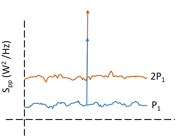
4. To determine the laser's power spectral density, we measure the laser power repeatedly, each time for a time $T$. The measured value will fluctuate with a standard deviation $\sigma_P$.
5. Our measurement bandwidth is given by the sample frequency $\frac{1}{T}$.
6. We can thus calculate the power spectral density of the laser power: $$S_{pp} = \frac{P \hbar \omega_0}{T} \cdot \frac{T}{1} = P \hbar \omega_0 \quad \big( \text{Watts}^2 / \text{Hz} \big)$$

2.2. Noise in sensors

So far, we have been talking about noise in a measurement. In sensing, typically one measures the "thing" we want to sense by translating it into a signal that one can record, like a voltage or a current. The device that converts the quantity that we want to measure, such as the position of an object or the power of a laser, into an observable signal is called a "sensor":

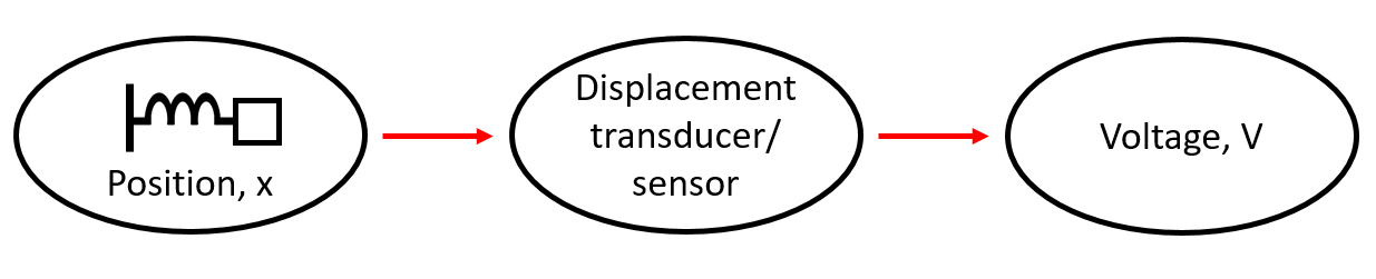
A sensor often produces an output that is linearly proportional to the input.

1. For example, if the sensors input is position $x$, and the output of the sensor is a voltage, then we would have:

   $$V = R x \quad R = \frac{dV}{dx}$$

   Here, we have defined a constant $R$ as the conversion factor, sometimes called "transduction gain", or also the "responsivity". In this example it could have units such as Volts / mm, describing how many volts the sensor outputs for a millimeter displacement of th object is measuring.

   More generally, the reponsivity $R$ is the proportionality constant (or slope) relating the signal out $S_out$ of the sensor to the signal coming into it $S_in$:

   $$R = \frac{dS_{out}}{dS_{in}}$$

2. Another example of a sensor could be, for example, a voltage amplifier which takes a voltage $V_{in}$ at its input and amplifies this to create a (larger) voltage at its output $V_{out}$:

   $$R = \frac{dV_{out}}{dV_{in}}$$

   Note that in this example, since the output and the input have the same units, the responsivity is in fact the voltage gain $G$ of the amplifier.

How sensitive is our sensor? A common mistake is to associate $R$ with the sensitivity, as in: "A photodetector with a larger Amps/Watt conversion factor is more sensitive".

If we define "sensitivity" as the ability to distinguish a small signal from the noise, then we can see that this is nonsense!

Why? Because our ability to distinguish signals from noise also depends on how much noise we have in the reading of our sensor: what we care about is the equivalent $\sigma_x$ given the amount of noise $\sigma_v$ we have in our recorded data. For the linear sensor described above, these are related as

$$\sigma_x = \frac{\sigma_v}{R_{vx}} = \frac{\sigma_v}{dV/dx}$$

Sensitivity

The sensitivity of our detector is determined by the power spectral density of its noise

$$S_{xx} = \frac{S_{vv}}{(R_{vx})^2}$$

Typically, when discussing sensors, people prefer to work with "sensitivity" defined as:

$$\sqrt{S_{xx}} = \frac{\sqrt{S_{vv}}}{R_{vx}}$$

For a sensor of position, the sensitivity $\sqrt{S_{xx}}$ has units of m/$\sqrt{Hz}$.

What does $\sqrt{S_{xx}}$ tell us? If $\sqrt{S_{xx}}$ = 1nm/$\sqrt{Hz}$, then it means if we average for 1 second, we will be able to detect a 1nm displacement signal with a signal to noise (SNR) ratio of 1:

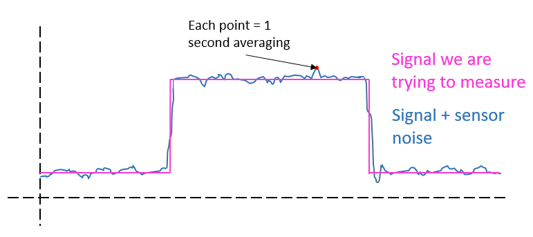
One slightly confusing point: better sensitivity is smaller $\sqrt{S_{xx}}$.

One last point: what if the relation between $x$ and $V$ is not linear? If the noise is small compared to the signal, then we can use the rules of error propagation to find the conversion of $\sigma_v$ into $\sigma_x$:

$$V = f(x)\\ \sigma_v = \frac{df}{dx} \sigma_x$$

It looks similar, but now the derivative may be dependent on the average value of $x$ (i.e. not just constant).

Conclusions

1. The central limit theorem tells us that the probability distribution of an infinite sum of independent random variables is Gaussian
2. A Poissonian probability distribution arises when events happen independently
3. The sensitivity of a detector is limited by the power spectral density of the detector noise