Lecture 4: Quantum fluctuations, the quantum harmonic oscillator, and coherent states

Expected prior knowledge

Before the start of this lecture, you should be able to:

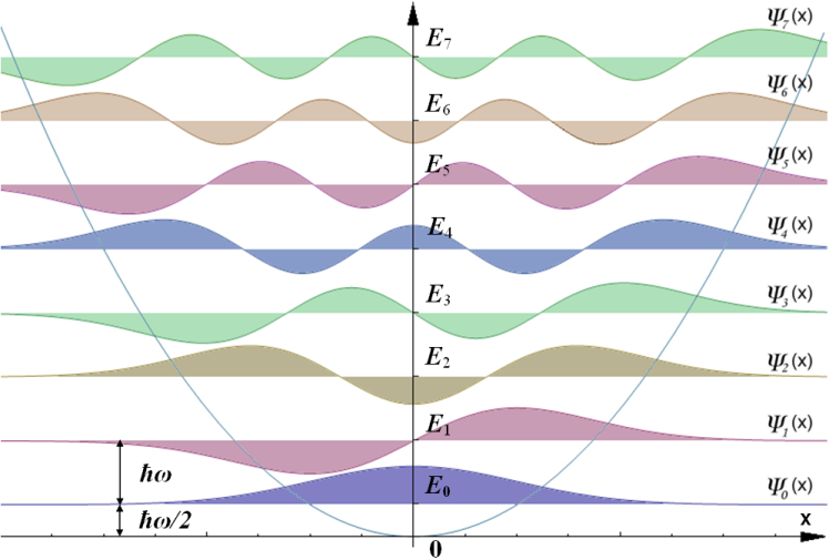
1. Write down the energy spectrum of the quantum harmonic oscillator
2. Recall that the state of a quantum object is described by the wavefunction $|\Psi\rangle$
3. Calculate the expectation value of an observable given a wavefunction
4. Write down and apply the Heisenberg x-p and the generalised uncertainty relations

Learning goals

After this lecture you will be able to:

1. Derive the quantum fluctuations for a given wavefunction
2. Calculate expectation values of coherent states
3. Show that the number of photons in a coherent state follows a Poisson distribution

---

So far, we have been reviewing concepts from classical noise, and discovering fun things like the fluctuation-dissipation theorem by accident. This week, we will start to explore fluctuations in quantum mechanics, using the harmonic oscillator as the core example. But first, we will review the uncertainty principle.

4.1. Review: The Heisenberg Uncertainty principle and quantum fluctuations

One of important concepts in quantum mechanics is the Heisenberg uncertainty principle.

In its more precise formulation, the uncertainty principle describes the relation between the uncertainties in position $x$ and momentum $p$ of a particle that arise from the Schroedinger wave equation.

The uncertainties we are talking about in this case are defined by expectations values calculated using the wavefuntion $\psi(x)$ of the particle:

$$\sigma_x = \sqrt{\langle x^2 \rangle - \left\langle x \right\rangle^2}$$

$$\sigma_p = \sqrt{\langle p^2 \rangle - \left\langle p \right\rangle^2}$$

The expectation values above are calculated using the wave function in the usual way, for example:

$$\langle p \rangle = \langle \psi | \hat p | \psi \rangle = \int \psi^*(x)\ (-i \hbar) \frac{d}{dx}\ \psi(x) dx$$

Quantum fluctuations

If one were to repeatedly prepare a particle in state $|\psi\rangle$ and perform a sequence of measurements of the particle's position, each of those measurements would (could) result in a different value, and the standard deviation of your measurement outcomes would be equal to $\sigma_x$ as calculated above. Because the outcome of each repeated measurement of position starting from the same initial wavefunction $|\psi\rangle$ is different, the consequence of a non-zero $\sigma_x$ is often referred to as the quantum fluctuations of the position of the particle associated with quantum state $|\psi\rangle$. Similarly, $\sigma_p$, representing the uncertainty of momentum encoded in a wave function, can also be referred to as the quantum fluctuations of the particle's momentum.

Quantum noise

Finally, the irregularity that quantum fluctuations introduce into a set of measurements can be referred to as quantum noise, and in general, the presence of non-zero quantum fluctuations / noise / uncertainty can have important physics consequences even if one does not collapse the wavefunction by performing a measurement.

Note: although quantum noise is frequently referred to as "fluctuations", keep in mind that there is nothing associated with the quantum states $|\psi\rangle$ that has to be changing in time. Quantum fluctuations do not "fluctuate in time". We will see an explicit example of this below: in particular, the stationary states (energy eigenstates) of the Harmonic oscillator are absolutely "stationary" in every sense; the expectation value of all operators in quantum mechanics do not change in time for a stationary state. Quantum fluctuations only "fluctuate" when a measurement apparatus breaks the evolution of the Schroedinger equation and collapses the wave function.

The (original) Heisenberg uncertainty principle places a lower limit on product of the quantum fluctuations of position and momentum:

$$\sigma_x \sigma_p \ge \frac{\hbar}{2}$$

This can also be understood intuitively from the Schroedinger wave equation: making a smaller wave packet in space $x$ requires higher spatial frequency components of the wave function, which, from the definition of the momentum operator, results in more uncertainty in the momentum.

The same concept is linked to "confinement energy": if I confine a particle to a fixed region of space of length $l$, for example by putting it in a box with an infinite square well potential or confine it using a harmonic $x^2$ potential, then the above relation also puts a lower bound (minimum) on $\sigma_p$:

$$\sigma_p \ge \frac{\hbar}{2l}$$

This lower bound on $\sigma_p$ is the physical origin of the "zero point" energy found in the ground state the harmonic oscillator, but also in the infinite square well, and in real physical systems like atoms. One can even use the above to make a decent estimate of the zero point (kinetic) energy. In the ground state, the particle is not "moving": it has not average momentum, so $\langle p \rangle = 0$. However, due to the uncertainty principle, we can then see that the expectation value of the square of the momentum is not zero:

$$\langle p^2 \rangle = \sigma_p^2 + \langle p \rangle^2 = \sigma_p^2 \ge \frac{\hbar^2}{4l^2}$$

We can then see that the particle must have some (expectation value of its) kinetic energy, since the kinetic energy operator $\hat E_{kin} = \hat T = \tfrac{1}{2m} \hat p^2$:

$$\langle E_{kin} \rangle = \frac{\langle p^2 \rangle}{2m} \approx \frac{\hbar^2}{8ml^2}$$

More review: Beyond $x$ and $p$: The generalised uncertainty principle

The "traditional" $x-p$ Heisenberg uncertainty principle is actually a specific example of a more generalised uncertainty principle that relates the minimum allowed uncertainty between two observables in quantum mechanics. This, along with a very enlightening expose of the real meaning of the "energy-time" uncertainty principle, is discussed in detail in chapter 3 of the book "Introduction to Quantum Mechanics by Griffiths.

In the most general case, the uncertainty principle for two observables $A$ and $B$ is given by:

$$\sigma_A^2 \sigma_B^2 \ge \left( \frac{1}{2i}\langle[\hat A, \hat B] \rangle \right)^2$$

For any two "compatible" observables whose operators $\hat A$ and $\hat B$ commute, the uncertainty limit says nothing useful: quantum mechanics places no constraint on how small the uncertainty one of these may be based on a given uncertainty in the other.

Note also that the expression above includes an expectation value:

$$\langle[\hat A, \hat B] \rangle = \langle \psi | \ (\hat A \hat B - \hat B \hat A) \ | \psi \rangle$$

So in general, the exact limit that uncertainty principle imposes will also depend on the specific quantum state $\psi$ you choose.

The $x-p$ uncertainty principle is a particularly simple example of the above. First, $x$ and $p$ do not commute, as we know, and so the constraint above will tell us something meaningful. Second of all, the commutator of $x$ and $p$ is a scalar:

$$[\hat x, \hat p] = i \hbar$$

which means that we can put it out of our braket above, being left with $\langle \psi | \psi \rangle = 1$. So it is also a particularly simple case where the limit that the uncertainty principle places is independent of the state you choose.

4.2. Quantum noise in a harmonic oscillator

Here, we will explore in more detail the types of quantum noise states can haveWe will start with a problem you have seen before: the quantum harmonic oscillator (i.e., a quantum mass on a spring).

Why is the quantum harmonic oscillator such an important concept?

• For small displacements from a minimum, all potentials are approximately harmonic (i.e., parabolic, via Taylor expansion)
• Electrical circuits can be harmonic oscillators
• Light and lattice vibrations are descirbed by harmonic oscillators

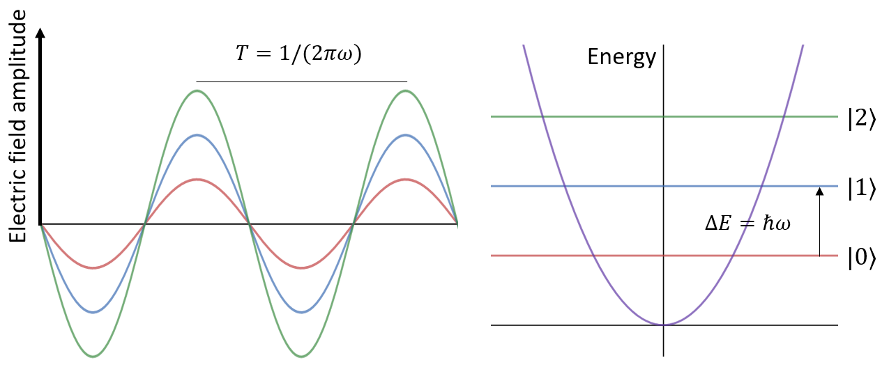
The last one is particularly interesting, and we can gain a deeper understanding of what "photons" are by looking at how light, and photons, are related to harmonic oscillators.

Imagine an empty box that contains electromagnetic radiation.

1. Classically, each mode of the box is a standing wave that bounces up and down in time:

   • mode $1$: $\quad E_1 \cos{(\omega_1 t)} \sin{(\frac{\pi x}{L})}$
   • mode $2$: $\quad E_2 \cos{(\omega_2 t)} \sin{(\frac{2 \pi x}{L})}$
   • mode $n$: $\quad E_n \cos{(\omega_n t)} \sin{(\frac{n \pi x}{L})}$

2. Associated with every electric field $\vec{E}$, there is a magnetic field $\vec{B}$ that oscillates out of phase with respect to the electric field (this follows from Maxwell's Equations).

3. The total energy is given by:

$$E = \frac{1}{2}\int (\epsilon_0 |\vec{E}|^2 + \mu_0 |\vec{B}|^2) d^3 x$$

1. For a given mode, this will be proportional to:

$$E_m \propto a E_m^2 + b B_m^2$$

1. This is looking a lot like a harmonic oscillator

$$E = \frac{1}{2} m \omega_0^2 x^2 + \frac{p^2}{2 m}$$ where the electric and magnetic fields play the roles of position and momentum, respectively.

1. Each mode of the box can be mapped to an individual harmonic oscillator. Each such oscillator can be quantized, and each mode can be excited by an arbitrary number of photons.

Having established the importance of the harmonic oscillator, let's look at the properties of some of its states.

• The ground state of the oscillator is the lowest-energy state allowed in quantum mechanics. Unlike in classical mechanics, the ground does not sit at the bottom of the potential. Instead, it has a zero-point energy of $\frac{1}{2}\hbar \omega$, where $\omega$ is the eigenfrequency of the oscilator.

• The ground-state wavefunction is "smeared out" in space, so there are zero-point fluctuations in the position of the oscillator. The standard deviation of the position is $x_\text{ZPF} = \sqrt{\frac{\hbar}{2 m \omega}}$.

What does it mean for the wavefunction to be "smeared out"?

• Since we interpret $|\Psi(x)|^2$ as a probability distribution, we can take a particle described by the wavefunction, measure its position, and then reset the particle. After many trials, the histogram of the random measurement results will converge to the distribution $\rho(x) = |\Psi(x)|^2$.

Let's take a step back, and pretend that we don't perform any measurements. Does any "property" of the particle in the ground state of the quantum harmonic oscillator change in time?

• Under the evolution of the Schr\"{o}dinger equation, we have

$$\Psi(x,t) = e^{i E_0 t / \hbar} \psi_0 (x)$$

So the total wavefunction $\Psi(x,t)$ changes in time only via an oscillating phase factor.

Do any observables change?

• It turns out that none of $\langle x \rangle, \langle p \rangle, \langle E_\text{pot} \rangle, \langle E_\text{kin} \rangle$ change in time. This is interesting, because if these quantities were associated with a classical oscillator, the finite energy would cause all of them to oscillate in time. Instead, in the quantum case, the particle has energy but these expectation values are stationary. Yes, there are fluctuations in the quantum sense, but these fluctuations themselves do not fluctuate in time. In fact, they only fluctuate if you measure them! (A philosophical aside: does it even make sense to talk about something of we are not allowed to measure it?)

So, if the oscillator is stationary, why does it have kinetic energy? - $$\langle E_\text{kin} \rangle = \frac{\langle p^2 \rangle}{2m} = \frac{\langle p \rangle^2}{2m} + \frac{\sigma_p^2}{2m}$$ The first term is energy associated with classical motion, and the second comes from quantum fluctuations.

So if all of the oscillator eigenstates are stationary, how can we get them to "move"?

• Suppose we prepare a superposition of two such states, like $|\Psi(t=0)\rangle=\frac{1}{\sqrt{2}}(|0\rangle + |1\rangle)$. This will evolve in time as

$$|\Psi(t)\rangle= \frac{1}{\sqrt{2}}(e^{-iE_0t/\hbar}|0\rangle + e^{-iE_1t/\hbar}|1\rangle).$$ The relative phase between the two states will cause the observable $\langle x(t) \rangle$ to oscillate in time.

4.3. Coherent states

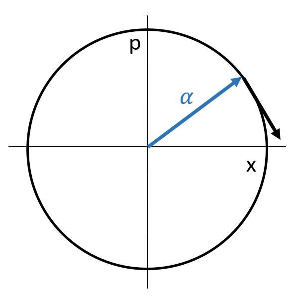
Another very important state of the quantum harmonic oscillator is the "coherent state" (see problem 3.35 from Griffiths). Mathematically, the coherent state is defined as

$$|\alpha\rangle = e^{-\frac{|\alpha|^2}{2}} \sum_{n=0}^{\infty} \frac{\alpha^n}{\sqrt{n!}} |n\rangle$$

where $\alpha$ is complex.

Properties of coherent states

The coherent state has the following properties:

1. The coherent state is not an eigenstate of the Hamiltonian. Therefore, generally, it will "move" (i.e., $\langle x \rangle$ and $\langle p \rangle$ oscillate in time).

2. Instead, the coherent state is an eigenstate of the annihilation operator $\hat{a}$.

   Creation and Annihilation operators

   Recall that the creation operator $\hat{a}^\dagger$ and the annihilation operator $\hat{a}$ have the following properties: $$\begin{align} \hat{a}|n\rangle = & \sqrt{n}|n-1\rangle \quad \text{and} \quad \hat{a}|0\rangle=0, \\ \hat{a}^\dagger|n\rangle = & \sqrt{n+1}|n+1\rangle,\\ \hat{a}^\dagger\hat{a}|n\rangle =& n|n\rangle. \end{align}$$ The last operator, $\hat{n}=\hat{a}^{\dagger}\hat{a}$, is called the number operator. It allows us to write the Hamiltonian as $\hat{H}=\hbar\omega(\hat{a}^\dagger\hat{a}+0.5)$. Comparing this to $$\hat{H}=\frac{\hat{p}^2}{2m}+\frac{1}{2}m\omega_0^2\hat{x}^2,$$ we can derive $$\begin{align} \hat{x} = &x_\text{ZPF}(\hat{a}^\dagger+\hat{a})\\ \hat{p} = & i\frac{\hbar}{2 x_\text{ZPF}}(\hat{a}^\dagger-\hat{a}). \end{align}$$

3. There are an infinite number of possible coherent states, since $\alpha$ can vary continuously: $\alpha = |\alpha|e^{i \theta}$.

4. All coherent states are Heisenberg-limited minimum uncertainty wavepackets that satisfy $\sigma_x \sigma_p = \frac{\hbar}{2}$ (see exercise).
5. As a function of time, a coherent state evolves into a new coherent state with the same amplitude but a different phase: $\alpha(t) = e^{-i \omega t} \alpha$.
6. The ground state $|0\rangle$ is also a coherent state, with $\alpha = 0$ and $\langle x \rangle = \langle p \rangle = 0$.
7. By expressing the operators for position and momentum in terms of creation and annihilation operators, it follows that a coherent state $\alpha$ has: $$\begin{align} \langle x \rangle &= x_{ZPF} (\alpha + \alpha^*) = 2 x_{ZPF} \mathcal{Re}(\alpha)\\ \langle p \rangle &= \frac{\hbar}{2 x_{ZPF}} \big( \frac{\alpha - \alpha^*}{i} \big) = \frac{\hbar}{x_{ZPF}}\mathcal{Im}(\alpha) \end{align}$$
8. Using the fact that $\alpha(t) = e^{-i \omega t} \alpha(0)$, we can see that the above expectation values oscillate in time.
   

   

   In quantum optics, $\hat{x}$ and $\hat{p}$ are called quadratures.
9. The photon number operator $\hat{n}$ is $\hat{a}^\dagger \hat{a}$ (i.e. $\langle n | \hat{n} | n \rangle = n$), and the Hamiltonian then becomes $\hat{H} = \hbar \omega (\frac{1}{2} + \hat{a}^\dagger \hat{a})$. Using this, we find that $$\langle \alpha | \hat{n} | \alpha \rangle = |\alpha|^2 = \bar{n}$$
10. It turns out that the variance of the number of photons in a coherent state, $\sigma_N^2$, is $|\alpha|^2$. The property that the variance is equal to the mean tells us that coherent states are Poissonian. If you recall that lasers are also described by Poissonian statistics, then we have found that lasers are actually just coherent states!

Coherent states have maximal "classical" energy, and even though they are (infinitely) large quantum superpositons, in some sense they are the most classical quantum states possible because they reach the limit of the smallest amount of quantum fluctuations allowed by the Heisenberg limit.

4.4. Conclusions

Conclusions

1. The expectation values of observables of stationary states do not depend on time.
2. However, there are quantum fluctuations. These are related to the spread/curvature of the wavefunction.
3. The coherent state is not a stationary state. Its time dynamics resemble that of a classical particle.
4. The coherent state is an eigenstate of the annihilation operator.
5. The expectation values for position and momentum of the coherent state $|\alpha\rangle$ can be expressed in terms of $\alpha$.