Lecture 7.1: The Density Matrix

Last lecture, we learned about continuous (i.e. weak) measurements in QM, which we can summarize as follows

1. In continuous measurements, collapse events occur randomly in time, following a Poisson distribution

2. At each collapse event, we apply the usual recipe for quantum measurement

3. The average rate at which the collapse events occur is proportional to how fast we (or other people) extract information about the observable we are observing

4. These collapse events result in "quantum backation" that disturbs the state we are measuring and can (but does not always) add noise to the observable we are measuring

We then saw a few examples

1. Noise in the oscillations of $\langle S_x(t) \rangle$ of a spin when measuring $S_x$

2. Noise in $\langle x(t) \rangle$ of a harmonic oscillator induced by measurements of $x$

Another example: measure $\langle n \rangle$ of a coherent state

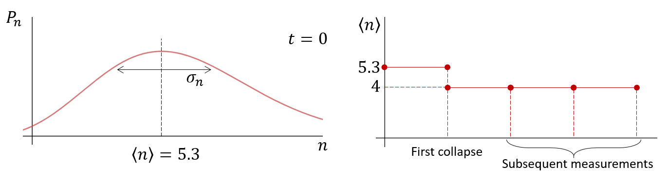
After the first collapse, $\langle n \rangle$ no longer changes in subsequent collapses. The reason is because the number operator $\hat{n}$ commutes with the Hamiltonian: $[\hat{n}, \hat{H}] = 0$. Thus, they share an eigenbasis, and upon measurement the system collapses to a stationary state, where $\langle n \rangle$ is not time-dependent. This is an example of a quantum non-demolition experiment. The first measurment always collapses $|\psi\rangle$, but the next measurements don't cause more "damage"; as a result, you can average stationary quantities for a long time, say, if your detector adds a lot of classical noise.

But there is a problem: what if we miss some of the measurement results, or our detector is noisy, giving us only partial information? Or even none at all?

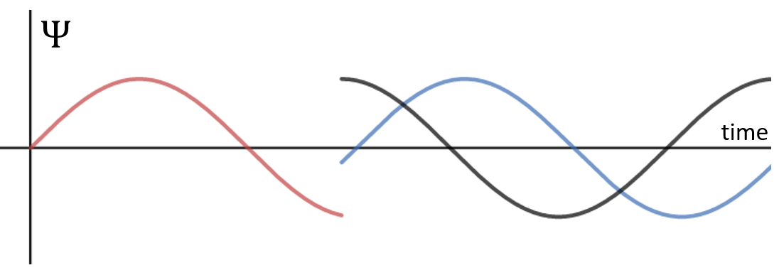
If our lack of information makes it ambiguous as to what state the system is in, then should we then keep track of two Schrodinger equations (like in the image)? Actually, in such a case, we would need to average over different collapse events in time, which is exactly what the Monte Carlo Wave Function (MCWF) method does, which we will see later in QuTip.

However, if we are only interested in the average result over different quantum trajectories, then we can just use the density matrix formalism.

Density matrix

The density matrix is defined as $$\rho = |\psi\rangle\langle\psi|$$ where $|\psi\rangle$ is some state (column) vector. We recall the usual inner product between state vectors $$\langle\psi|\psi\rangle = \sum_i |c_i|^2$$ which is a scalar quantity.

But what does it mean to reverse this notation, as in the definition of a density matrix? Writing $|\psi\rangle\langle\psi|$ is called an outer product, and instead of a scalar, it is a matrix: $$|\psi\rangle\langle\psi| = \begin{bmatrix} c_1 \\ c_2 \\ c_3 \\ \vdots \end{bmatrix} \begin{bmatrix} c_1^* & c_2^* & c_3^* & \dots \end{bmatrix} = \begin{bmatrix} c_1 c_1^* & c_1 c_2^* & c_1 c_3^* & \dots \\ c_2 c_1^* & c_2 c_2^* & c_2 c_3^* & \dots \\ c_3 c_1^* & c_3 c_2^* & c_3 c_3^* & \dots \\ \vdots & \vdots & \vdots & \ddots \\ \end{bmatrix}$$

Some properties of $\rho$: $$\begin{aligned} Tr(\rho) &= \sum_i |c_i|^2 = 1\\ \rho_{ij} &= \rho_{ji} \quad (\text{Hermitian}) \end{aligned}$$

Example: Spin-$1/2$

The typical example is spin-$1/2$: $$\begin{align} |\psi\rangle &= |\uparrow\rangle = \begin{bmatrix} 1 \\ 0 \end{bmatrix} \rightarrow \rho = \begin{bmatrix} 1 & 0 \\ 0 & 0 \end{bmatrix} \rightarrow Tr(\rho) = 1 + 0 = 0\\ |\psi\rangle &= |y+\rangle = \frac{1}{\sqrt{2}}\begin{bmatrix} 1 \\ i \end{bmatrix} \rightarrow \rho = \begin{bmatrix} 1/2 & -i/2 \\ i/2 & 1/2 \end{bmatrix} \rightarrow Tr(\rho) = 1/2 + 1/2 = 1 \end{align}$$

Now we need to keep track of $N^2$ numbers in matrix instead of $N$ in a vector, so what is the benefit? For one, there is a very handy expression for expectation values:

$$\langle A \rangle = Tr(\rho A)$$

A few examples of using this nice trace formula:

$$\begin{align} S_Z, |\uparrow\rangle &\rightarrow Tr \bigg( \frac{\hbar}{2}\begin{bmatrix} 1 & 0 \\ 0 & 0 \end{bmatrix} \bigg) = \frac{\hbar}{2}\\ S_Y, |\uparrow\rangle &\rightarrow Tr \bigg( \frac{\hbar}{2}\begin{bmatrix} 0 & i \\ 0 & 0 \end{bmatrix} \bigg) = 0\\ S_Z, |y+\rangle &\rightarrow Tr \bigg( \frac{\hbar}{4}\begin{bmatrix} 1 & -i \\ -i & -1 \end{bmatrix} \bigg) = 0\\ S_Y, |y+\rangle &\rightarrow Tr \bigg( \frac{\hbar}{4}\begin{bmatrix} 1 & -i \\ i & 1 \end{bmatrix} \bigg) = \frac{\hbar}{2} \end{align}$$

Mixed and pure states

The time-dependent Schrodinger equation (TDSE) also takes on a compact form:

$$i\hbar \frac{\partial \rho}{\partial t} = [\hat{H}, \rho]$$

But how does this help with the collapse problem? The key concept is that $\rho$ can allow us to include classical uncertainty into our quantum calculations.

Let's say that we do not know the exact state of the quantum particle, but we know that there is a 50% chance it is in state $|\psi_1\rangle$ and 50% chance it is in $|\psi_2\rangle$. The density matrix for this situation is

$$\begin{align} \rho &= \sum_i p_i |\psi_i\rangle\langle\psi_i|\\ &= 0.5|\psi_1\rangle\langle\psi_1| + 0.5 |\psi_2\rangle\langle\psi_2| \end{align}$$

This kind of density matrix is called a "mixed state" (or more appropriately, but less commonly, a "mixed ensemble"), in contrast to the case where there is only one term in the sum, which is called a pure state and was the first example we saw.

We can use the same formula above to calculate an "ensemble" expectation value of an observable:

$$\langle A \rangle = Tr(\rho A)$$

For pure states, this has the usual meaning of preparing a state $|\psi\rangle$, measuring the observable $\hat{A}$, and repeating this process to build up an average measurement result $\langle A \rangle$.

For mixed states, the process is a bit different. We do not prepape the same state each time, since we need to import classical uncertainty into the process. Each new $|\psi\rangle$ is either $|\psi_1\rangle$ or $|\psi_2\rangle$ with probability 50% for each (we can just flip a coin to decide). The uncertainty in our measurement results has two distinct origins: there is fundamental "quantum" randomness from the collapse of the wavefunction, and also boring "classical" randomness from the coin flip that decides the state preparation.

Let's assume the mixed state is split 50-50 between spin-up and spin-down, that is, $|\psi_1\rangle =|\uparrow\rangle$ and $|\psi_2\rangle =|\downarrow\rangle$. If we measure the observable $S_Z$, we would expect to get either up or down about half the time on average.

What if we had instead used the pure state $|+i\rangle\langle +i|$? We would get the same measurment statistics! But surely these states aren't the same, so how can we tell the difference? The answer to this question is, at its core, what makes quantum quantum.

If we instead measure the observable $S_Y$, the mixed state will still yield 50-50 results because either of its two states can be written as superpositions between the $|\pm i \rangle$ eigenstates. However, the pure state $|+i\rangle$ obviously will only ever give $+\hbar/2$ upon measuring the observable $S_Y$. This difference can be visualized with the density matrix

$$\begin{align} 0.5|\uparrow\rangle\langle\uparrow| + 0.5|\downarrow\rangle\langle\downarrow| &= \begin{bmatrix} \frac{1}{2} & 0 \\ 0 & \frac{1}{2} \end{bmatrix}\\ |+i\rangle\langle +i| &= \begin{bmatrix} \frac{1}{2} & \frac{-i}{2} \\ \frac{i}{2} & \frac{1}{2} \end{bmatrix} \end{align}$$

where the diagonal terms are called weights or populations, and the off-diagonal terms are called coherences. Mixing states suppresses the off-diagonal terms. We can check how pure a state is by computing its "purity"

$$\gamma = Tr(\rho^2)$$

If the state is pure, then squaring $\rho$ won't change the fact that its trace is $1 + 0 = 1$. But if some diagonal element is less than 1, then squaring the matrix will reduce the trace.

Lastly, the Wigner functions we saw earlier (for pure states) can also be used to encode classical uncertainty, like the density matrix. If we have a density matrix (pure or mixed), then its Wigner function is

$$W(x,p) = \frac{1}{\pi \hbar} \int_{-\infty}^{+\infty} \langle x+y | \rho | x-y \rangle e^{-2ipy/\hbar} dy$$

where $|x\rangle$ are the eigenstates of the position operator, expressed in whatever basis was chosen for $\rho$.

From the above, we can see that Wigner functions of mixed states have an interesting property: unlike the Wigner functions of superposition states, the Wigner functions of mixed states do add:

$$\begin{align} \rho_{mix} &= \rho_1 + \rho_2\\ W_{mix} &= \frac{1}{\pi \hbar} \int_{-\infty}^{+\infty} \langle x+y | \rho_1 | x-y \rangle e^{-2ipy/\hbar} dy\\ &+ \frac{1}{\pi \hbar} \int_{-\infty}^{+\infty} \langle x+y | \rho_2 | x-y \rangle e^{-2ipy/\hbar} dy \\ &= W_1 + W_2 \end{align}$$