Lecture 6: Quantum Measurement Backaction

Learning goals

After this lecture you will be able to:

1. Predict what outcomes of a quantum measurement could be
2. Discuss the concept of quantum backaction
3. Describe the time dynamics of a quantum state before and after a measurement

---

In this lecture, we will explore the concept of "quantum backaction", the idea in QM that measurement always induces some "action" on the state you are measuring.

This is also something that occurs in classical mechanics: if we measure the position of something with a camera, we need to use the flash to bounce some light off of it. Even classically, the electromagnetic waves from the flash will impart some momentum impulse on the thing we are taking a picture of, "kicking" it by a very small amount. In principle, in classical mechanics, this impulse from the flash can be known with infinite accuracy, and we can compensate for it and determine the position of our object with theoretically infinite precision. We could also determine its momentum at the same time by measuring the Doppler shift of the light from our flash.

The key difference in QM in this example is that the electromagnetic field from our flash necessarily contains quantum uncertainty, which will both limit how accurately we can measure the position (known as "quantum imprecision noise") and also give rise to quantum uncertainty in the force the light exerts on the object when it bounces (what we will call "quantum backaction noise").

While it would seem at first that these two are unrelated, in QM they are fundamentally connected: there is a minimum allowable disturbance of the object determined by how much information we acquire about it.

Furthermore, the nature of the backaction of your measurement itself, and the way it affects the noise you observe in subsequent measurements, depends on exactly what you measure.

In this lecture, we will try to illustrate some simple examples of these concepts without any mathematical formalism, which will be deferred to the next two lectures.

6.1. Review: Quantum Measurement and the generalised statistical interpretation

Before we start, we should review the generalized statistical interpretation of QM. If we want to predict what happens when we make a measurement:

1. Find the eigenstates and eigenvalues $|\lambda_A\rangle$, $\lambda_A$ of some observable $\hat{A}$

2. The measurement outcome is one such $\lambda_A$

3. The measurement outcomes are stochastic and the probability of finding value $\lambda_A$ is given by $|\langle \lambda_A | \psi \rangle|^2$, where $\hat{A}|\lambda_A\rangle = \lambda_A|\lambda_A\rangle$

4. After measurement with outcome $\lambda_A$, the state collapses to $|\lambda_A\rangle$ and subsequently continues to evolve according to the time-dependent Schrodinger equation (TDSE).

• What happens if we measure again?
• In particular, if we measure continuously as a function of time, how does the state evolve?
• If we just "look" at our quantum object, what happens?
• What does continuous measurement even mean?

Surely we cannot just continuously and instantaneously collapse the wavefunction, or else we could prevent objects from moving just by looking at them.

So, if we are looking "all the time", how often does the wavefunction collapse?

1. The collapse occurs randomly in time

2. It happens at an average "collapse rate" determined by how quickly I obtain information about the thing I am observing

The greater the signal-to-noise ratio our detector provides, the faster the average collapse rate. Note that this means that collapse is a Poissonian process!

Point 2 above assumes that we are the only observers, and that none of the quantum information is leaking out to the environment, which is almost never the case. In almost all experiments there is some loss of information about the quantum state into a "bath" that we don't have access to. In this case, Point 2 should be amended to

2.(revised) Collapse events occur at a rate determined by the rate of leakage of information out of the quantum state of the object we are obersving (including both our measurement rate and that of all others in the environment)

Let's take a look at a toy example: the measurement of the position of a harmonic oscillator that starts in its ground state. We will measure its position.

Upon measurement, its wavefunction collapses to a $\delta$-function! What will happen to $\langle x(t) \rangle$ after the collapse occurs?

• Since a $\delta$-function is not a stationary state, it will "move", and $\langle x(t) \rangle$ will depend on time

• What is the energy after we have measured? It should be higher than the ground state energy.

As a result of measurement, the mass will experience a random fluctuating force that increases with the strength of our measurement.

• This is called quantum backaction force and the resulting noise in $\langle x(t) \rangle$ is called quantum backation noise, or sometimes collapse noise

if we have complete information about the results of our measurements, this quantum backation noise is not random, and we can completely reconstruct it based on the measurement and thus predict how the mass will move! However, if some information is lost (perhaps in amplifier noise, or due to somebody else measuring and hiding their results) then this quantum backation noise will appear completely random to us.

6.2. The standard quantum limit (in optomechanics)

We have talked previously about laser interferometers and the sensitivity one would need to detect thermomechanical motion.

One of the striking features of QM is the prediction that even if we cool a vibrating object to absolute zero, it will still be "moving" due to zero-point fluctuations. As we saw earlier, one easy way to remember how big are these fluctuations is to apply the equipartition theorem but replace $\frac{1}{2}kT$ with $\frac{1}{2}E_0 = \frac{1}{4}\hbar\omega$:

$$\frac{1}{2}m\omega^2 x^2_{ZPF} = \frac{1}{4}\hbar\omega \rightarrow x_{ZPF} = \sqrt{\frac{\hbar}{2m\omega}}$$

Now, as experimentalists, we might ask whether we can build something to measure this.

To answer this properly, we need to figure out the power spectral density of these fluctuations.

• Just like in the classical case $$S_{xx}^{ZPF} = \frac{x_{ZPF}^2}{\pi\gamma} = \frac{x_{ZPF}^2}{\pi\omega_0}Q$$

• Just like in the classical case, the higher the Q-factor, the easier it is to measure quantum fluctuations.

To detect these quantum fluctuations, it is common to use a laser interferometer.

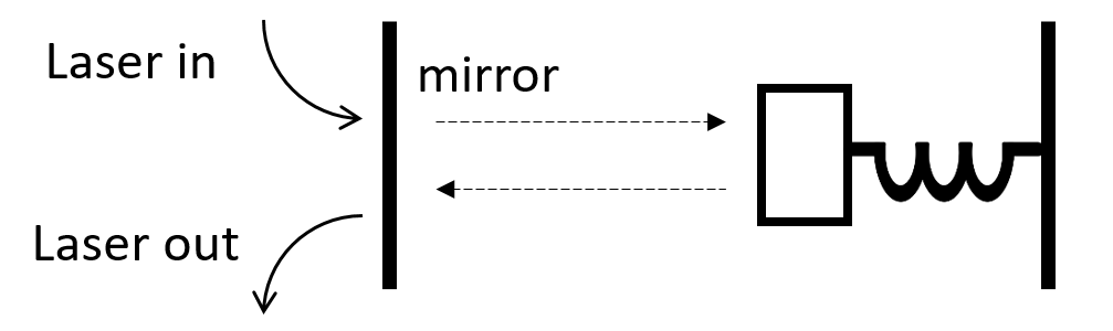
As we know, we can always increase the position sensitivity of a laser interferometer by turning up the laser power (in principle, though, in real life the laser power can be limited by boring things like absorption heating and melting mirrors). But ignoring these issues, we can theoretically just turn up the laser, decreasing the (squared) sensitivity of the laser detector because $S_{xx}^{det} \propto \frac{1}{P}$ until it is smaller than $S_{xx}^{ZPF}$ and then directly observe quantum fluctuations.

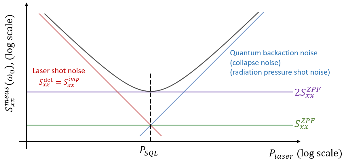
It almost seems like a conspiracy: the laser shot noise and quantum backaction noise cross exactly where we might be able to observe the zero-point fluctuations! Of course, it is not actually a coincidence; they cross there because that is exactly the point at which you begin to get sufficient information to collapse the wavefunction before the quantum motion "decays" (or, more precisely, before it "decoheres", determined by the autocorrelation function of our device $\propto \frac{1}{\gamma}$).

Finally, the two noise curves in the above plot look very different in the $S_{xx}^{meas}(\omega)$ spectrum.

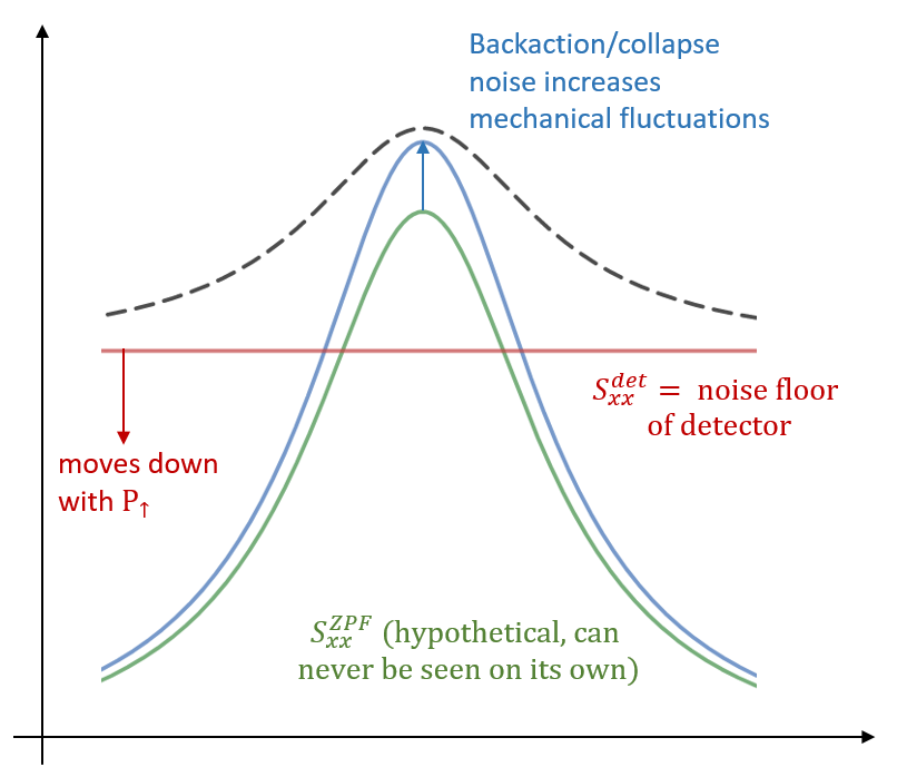
• $S_{xx}^{det}$ is the white detector noise floor from the added noise in your laser detection system,
• while $S_{xx}^{ZPF}$ and the backaction noise are Lorentzian noise peaks associated with actual mechanical motion.